Usage

Input/Output files

Input and output files in caspo are mostly comma separated values (csv) files. Next, we describe all files either consumed or produced when running caspo subcommands.

Prior knowledge network

A prior knowledge network (PKN) is given using the simple interaction format (SIF). Lines in the SIF file must specify a source node, an edge sign (1 or -1), and one target node. Note that SIF format specification also consider several target nodes per line but this is not supported in caspo at the moment. In the example shown below we would say that a and b have a positive influence over d while c has a negative influence over d.

a	1	d
b	1	d
c	-1	d
b	1	e
c	1	e

Experimental setup

An experimental setup is given using the JSON format. The JSON file must specify three list of node names, namely, stimuli, inhibitors, and readouts. In the following example, a, b, and c are stimuli, d is an inhibitor while f and g are readouts.

{
  "stimuli": ["a", "b", "c"],
  "inhibitors": ["d"],
  "readouts": ["f", "g"]
}

Experimental dataset

A phospho-proteomics dataset is given using the MIDAS format. Notably, MIDAS format considers time-series data but as we will see later, caspo always requires the user to define the time-point of interest when reading a MIDAS file (see Learn). Different time-points of data acquisition are specified in columns with prefix DA:.

In the example shown below, looking at the third row we would say that, when a and c are present, i.e. stimulated, and d is not inhibited, i.e., the inhibitor of d is not present, readouts for f and g at time-point 10 are 0.9 and 0, respectively. Meanwhile, looking at the four row we would say that when a and c are present and d is inhibited (the inhibitor of d it is present), readouts for f and g at time-point 10 are 0.1 and 0.9, respectively.

TR:Toy:CellLine	TR:a	TR:b	TR:c	TR:di	DA:f	DA:g	DV:f	DV:g
1	1	0	1	0	0	0	0	0
1	1	0	1	1	0	0	0	0
1	1	0	1	0	10	10	0.9	0
1	1	0	1	1	10	10	0.1	0.9

Logical networks

Logical networks are given using a csv file as follows. We assume that every logical mapping in a given network is in disjunctive normal form (DNF). Thus, columns header specify all possible conjunctions targeting any given node, e.g. d<-a+!c (d equals a AND NOT c). Then, each row describes a logical network by specifying which conjunctions are present (1) in the network or not (0). Whenever, two conjunctions targeting the same node are present in a given network they are connected using OR. For example, if we look at the first row in the example below, since d<-a and d<-b+!c are both present, the complete logical mapping for d would be: d equals a OR (b AND NOT c).

Additional columns could be included to give more details related to each network, e.g., MSE, size, or the number of networks having the same input-output behavior. See the output csv files in subcommands Learn (networks.csv) or Classify (behaviors.csv). However, when parsing a csv file of logical networks, caspo ignores columns that cannot be parsed as logical mappings except for a column named networks which is interpreted as the number of networks exhibiting the same input-output behavior (including the representative network being parsed). In particular, such a column will be relevant when computing weighted average predictions (see Predict).

e<-c	e<-b	d<-a	d<-!c	d<-b	d<-a+!c	d<-b+!c	f<-d+e
1	1	1	0	0	0	1	0
1	1	1	1	0	0	0	0
1	1	1	0	1	0	1	0
1	1	1	1	1	0	0	0
1	1	1	0	0	0	1	0

Basic statistics over a family of logical networks are described using a csv file as follows. For each logical mapping conjunction we compute its frequency of occurrence over all logical networks in the family. Also, mutually exclusive/inclusive pairs of mapping conjunctions are identified.

mapping	frequency	exclusive	inclusive
e<-c	1.0000
e<-b	1.0000
d<-a	1.0000
d<-b+!c	0.6000	d<-!c
d<-!c	0.4000	d<-b+!c
d<-b	0.4000

Experimental designs

An experimental design is essentially a set of experimental perturbations, i.e., various combinations of stimuli and inhibitors. But also, we describe an experimental design by how its perturbations discriminate the family of input-output behaviors (see Design for an example visualization). Experimental designs are given using a csv file as shown below. A column named id is used to identify rows corresponding to the same experimental design. Next, columns with prefix TR: correspond to experimental perturbations in the same way as in MIDAS format. Finally, for each combination of stimuli and inhibitors in a given experimental design, we count pairwise differences generated over specific readouts (columns with prefix DIF:) and pairs of behaviors being discriminated by at least one readout (column named pairs).

In the example below we show one experimental design made of two experimental perturbations. The first perturbation requires b and c to be stimulated, it generates 2 pairwise differences over f, and it discriminates 2 pairs of behaviors. The second perturbation requires b to be stimulated and d to be inhibited, it generates 1 pairwise difference over f, 1 pairwise difference over g, and it discriminates 1 pair of behaviors.

id	TR:a	TR:b	TR:c	TR:di	DIF:f	DIF:g	pairs
0	0	1	1	0	2	0	2
0	0	1	0	1	1	1	1

Logical predictions

Based on the input-output classification (see Classify), we can compute the response of the system for every possible perturbation by combining the ensemble of predictions from all input-output behaviors. Thus, predictions of a logical networks family are given using a csv file as the (incomplete) example below. For each possible combination of stimuli and inhibitors (columns with prefix TR:), the prediction for any readout node will be the weighted average (columns with prefix AVG:) over the predictions from all input-output behaviors and where each weight corresponds to the number of networks exhibiting the corresponding behavior. Also, the mean variance over all predictions is computed (columns with prefix VAR:). See Predict for an example visualization of readout mean variances.

TR:a	TR:c	TR:b	TR:di	AVG:g	AVG:f	VAR:g	VAR:f
1	0	0	0	0.0	0.0	0.0	0.0
0	1	0	0	0.0	0.0	0.0	0.0
0	0	1	0	1.0	0.8	0.0	0.16
0	1	1	0	0.0	0.4	0.0	0.24

Intervention scenarios

An intervention scenario is simply a pair of constraints and goals over nodes in a logical network. Thus, intervention scenarios are given using a csv file as shown below. Each column specifies either a scenario constraint (SC:) or a scenario goal (SG:) over any node in the network. Next, each row in the file describes a different intervention scenario. Values can be either 1 for active, -1 for inactive, or 0 for neither active nor inactive. That is, a 0 means there are no constraint nor expectation over that node in the corresponding scenario.

In the example below, we show two intervention scenarios. The first scenario requires that both, f and g to reach the inactive state under the constraint of a being active. The second scenario required only f to reach the active state under no constraints.

SC:a	SG:f	SG:g
1	-1	-1
0	1	0

Intervention strategies

An intervention strategy is a set of Boolean interventions over nodes in a logical network. Thus, intervention strategies are given using a csv file as shown below. Each column specifies a Boolean intervention over a given node (prefix TR: is used for consistency with MIDAS and other csv files). Next, each row in the file describes a different intervention strategy. Values can be either 1 for active, -1 for inactive, or 0 for neither active nor inactive. That is, a 0 means there is no intervention over that node in the corresponding strategy.

TR:c	TR:b	TR:e	TR:d
0	0	-1	0
-1	-1	0	0
1	0	0	-1

Basic statistics over a set of intervention strategies are described using a csv file as follows. For each Boolean intervention we compute its frequency of occurrence over all strategies in the set. Also, mutually exclusive/inclusive pairs of interventions are identified.

intervention	frequency	exclusive	inclusive
c=-1	0.3333		b=-1
c=1	0.3333		d=-1
b=-1	0.3333		c=-1
e=-1	0.3333
d=-1	0.3333		c=1

Command Line Interface

The command line interface (CLI) of caspo offers various subcommands:

• learn: for learning a family of (nearly) optimal logical networks
• classify: for classifying a family of networks wrt their I/O behaviors
• design: for designing experiments to discriminate a family of I/O behaviors
• predict: for predicting based on a family of networks and I/O behaviors
• control: for controlling a family of logical networks in several intervention scenarios
• visualize: for basic visualization of the subcommands outputs
• test: for running all subcommands using various examples

Next, we will see how to run each subcommand and describe their outputs.

If you haven’t done it yet, start by asking caspo for help:

$ caspo --help
usage: caspo [-h] [--quiet] [--out O] [--version]
             {learn,classify,predict,design,control,visualize,test} ...

Reasoning on the response of logical signaling networks with ASP

optional arguments:
  -h, --help            show this help message and exit
  --quiet               do not print anything to standard output
  --out O               output directory path (Default to './out')
  --version             show program's version number and exit

caspo subcommands:
  for specific help on each subcommand use: caspo {cmd} --help

  {learn,classify,predict,design,control,visualize,test}

Learn

This subcommand implements the learning of logical networks given a prior knowledge network and a phospho-proteomics dataset [1, 2]. In order to account for the noise in experimental data, a percentage of tolerance with respect to the maximum fitness can be used, e.g., we use 4% in the example below. Analogously, in order to relax the parsimonious principle a tolerance with respect to the minimum size (networks complexity) can be used as well. Further, other arguments allow for controlling the data discretization or the maximum number of inputs per AND gate.

Help on caspo learn:

$ caspo learn --help
usage: caspo learn [-h] [--threads T] [--conf C] [--fit F] [--size S]
                   [--factor D] [--discretization T] [--length L]
                   pkn midas time

positional arguments:
  pkn                 prior knowledge network in SIF format
  midas               experimental dataset in MIDAS file
  time                time-point to be used in MIDAS

optional arguments:
  -h, --help          show this help message and exit
  --threads T         run clingo with given number of threads
  --conf C            threads configurations (Default to many)
  --optimum O         logical network in CSV format. If many networks are
                      given, the first network is used (If given, avoids
                      learning the optimum and go directly to enumeration)
  --fit F             tolerance over fitness (Default to 0)
  --size S            tolerance over size (Default to 0)
  --factor D          discretization over [0,D] (Default to 100)
  --discretization T  discretization function: round, floor, ceil (Default to
                      round)
  --length L          max conjunctions length (sources per hyperedges)
                      (Default to 0; unbounded)

Run caspo learn:

$ caspo learn pkn.sif dataset.csv 30 --fit 0.04

Running caspo learn...
Number of hyperedges (possible logical mappings) derived from the compressed PKN: 130
Optimum logical network learned in 1.0537s
Optimum logical networks has MSE 0.0499 and size 28
2150 (nearly) optimal logical networks learned in 2.6850s
Weighted MSE: 0.0513

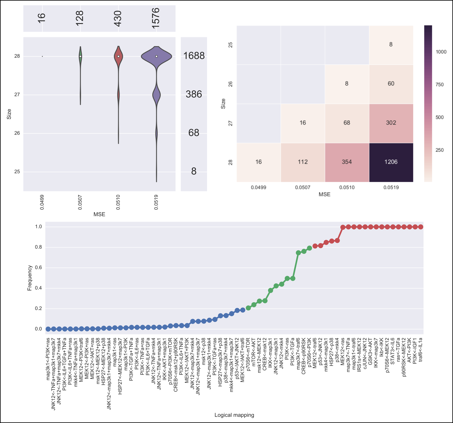
The output of caspo learn will be two csv files, namely, networks.csv and stats-networks.csv. The file networks.csv describes all logical networks found with their corresponding MSE and size. The file stats-networks.csv describes the frequency of each logical mapping conjunction over all networks together with pairs of mutually inclusive/exclusive mappings. The weighted MSE combining all networks is also computed and printed in the standard output.

In addition, the following default visualizations are provided describing the family of logical networks. At the top, we show two alternative ways of describing the distribution of logical networks with respect to MSE and size. At the bottom, we show the (sorted) frequencies for all logical mapping conjunctions.

Classify

This subcommand implements the classification of a given family of logical networks with respect to their input-output behaviors [1]. Notably, the list of networks generated by caspo learn can be used directly as the input for caspo classify.

Help on caspo classify:

$ caspo classify --help
usage: caspo classify [-h] [--threads T] [--conf C] [--midas M T]
                      networks setup

positional arguments:
  networks     logical networks in CSV format
  setup        experimental setup in JSON format

optional arguments:
  -h, --help   show this help message and exit
  --threads T  run clingo with given number of threads
  --conf C     threads configurations (Default to many)
  --midas M T  experimental dataset in MIDAS file and time-point to be used

Run caspo classify:

$ caspo classify networks.csv setup.json --midas dataset.csv 30

Running caspo classify...
Classifying 2150 logical networks...
31 input-output logical behaviors found in 156.9032s
Weighted MSE: 0.0513

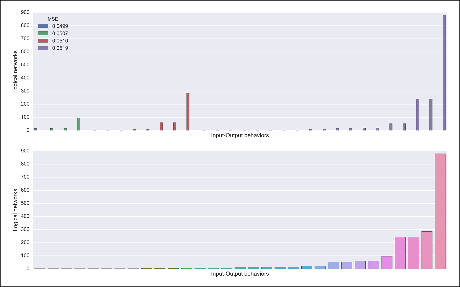
The output of caspo classify will be a csv file named behaviors.csv describing one representative logical network for each input-output behavior found among given networks. For each representative network, the number of networks having the same behavior is also given. Further, if a dataset is given, the weighted MSE is computed.

Also, one of the following visualizations is provided depending on whether the dataset was given as an argument or not. If the a dataset is given, the figure at the top is generated where I/O behaviors are grouped by MSE to the given dataset. Otherwise, the figure at the bottom is generated.

Design

This subcommands implements the design of novel experiments in order discriminate a given family of input-output behaviors [3]. Notably, the list of input-output behaviors generated by caspo classify can be used directly as the input for caspo design. Further, other arguments allow for controlling the maximum number of stimuli and inhibitors used per experimental condition, or the maximum number of experiments allowed.

Help on caspo design:

$ caspo design --help
usage: caspo design [-h] [--threads T] [--conf C] [--stimuli S]
                    [--inhibitors I] [--nexp E] [--list L] [--relax]
                    networks setup

positional arguments:
  networks        logical networks in CSV format
  setup           experimental setup in JSON format

optional arguments:
  -h, --help      show this help message and exit
  --threads T     run clingo with given number of threads
  --conf C        threads configurations (Default to many)
  --stimuli S     maximum number of stimuli per experiment
  --inhibitors I  maximum number of inhibitors per experiment
  --nexp E        maximum number of experiments (Default to 10)
  --list L        list of possible experiments
  --relax         relax full pairwise discrimination (Default to False)

Run caspo design:

$ caspo design behaviors.csv setup.json

Running caspo design...
1 optimal experimental designs found in 219.5648s

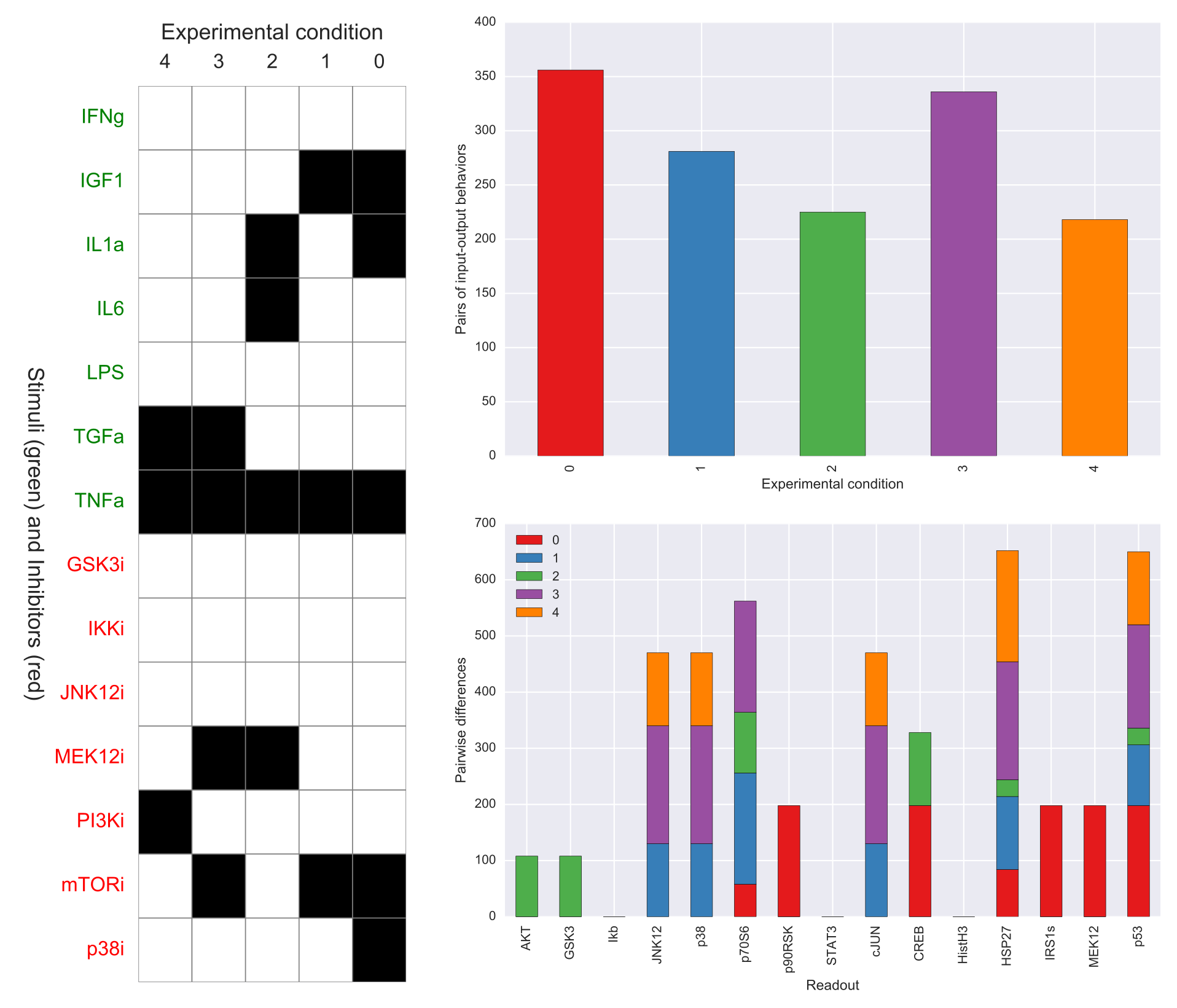
The output of caspo design will be one csv file, namely, designs.csv, describing all optimal experimental designs. In addition, the following visualizations are provided for each experimental design in such a file. At the left we show all experimental conditions for each experimental design. At the top right we show the number of pairs of I/O behaviors discriminated by each experimental condition. At the bottom right we show the number of pairwise differences over specific readouts by each experimental condition.

Predict

This subcommands implements the prediction of all possible experimental condition using the ensemble of predictions from a given family of logical networks. Since predictions are based on a weighted average, a variance can also be computed to investigate the variability on every prediction. Again, the list of input-output behaviors generated by caspo classify can be used directly as the input for caspo predict. In fact, any list of logical networks could be used. However, it is recommended to use a list of representative logical networks (with their corresponding number of represented networks) for better performance.

Help on caspo predict:

$ caspo predict --help
usage: caspo predict [-h] networks setup

positional arguments:
  networks    logical networks in CSV format.
  setup       experimental setup in JSON format

optional arguments:
  -h, --help  show this help message and exit

Run caspo predict:

$ caspo predict behaviors.csv setup.json

Running caspo predict...
Computing all predictions and their variance for 31 logical networks...

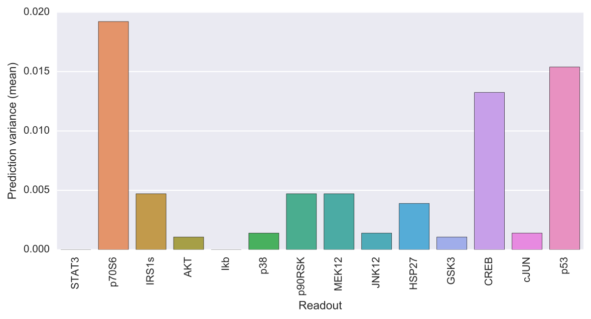
The output of caspo predict will be a csv file named predictions.csv describing for each possible experimental perturbation, the corresponding weighted average prediction and its variance for each readout. Also, the following visualization is provided showing the mean prediction variance for each readout over all possible experimental perturbations.

Control

This subcommand implements the control of a family of logical networks in terms of satisfying several intervention scenarios [4]. That is, it will find all intervention strategies for the given scenarios which are valid in every logical network in the family. Notably, the list of logical networks generated by caspo learn can be used directly as the input for caspo control. Further, other arguments allow for controlling the maximum number of interventions per strategy or whether interventions are allowed over constraints or goals.

Help on caspo control:

$ caspo control -h
usage: caspo control [-h] [--threads T] [--conf C] [--size M]
                     [--allow-constraints] [--allow-goals]
                     networks scenarios

positional arguments:
  networks             logical networks in CSV format
  scenarios            intervention scenarios in CSV format

optional arguments:
  -h, --help           show this help message and exit
  --threads T          run clingo with given number of threads
  --conf C             threads configurations (Default to many)
  --size M             maximum size for interventions strategies (Default to 0
                       (no limit))
  --allow-constraints  allow intervention over side constraints (Default to
                       False)
  --allow-goals        allow intervention over goals (Default to False)

Run caspo control:

$ caspo control networks.csv scenarios.csv

Running caspo control...
30 optimal intervention strategies found in 9.2413s

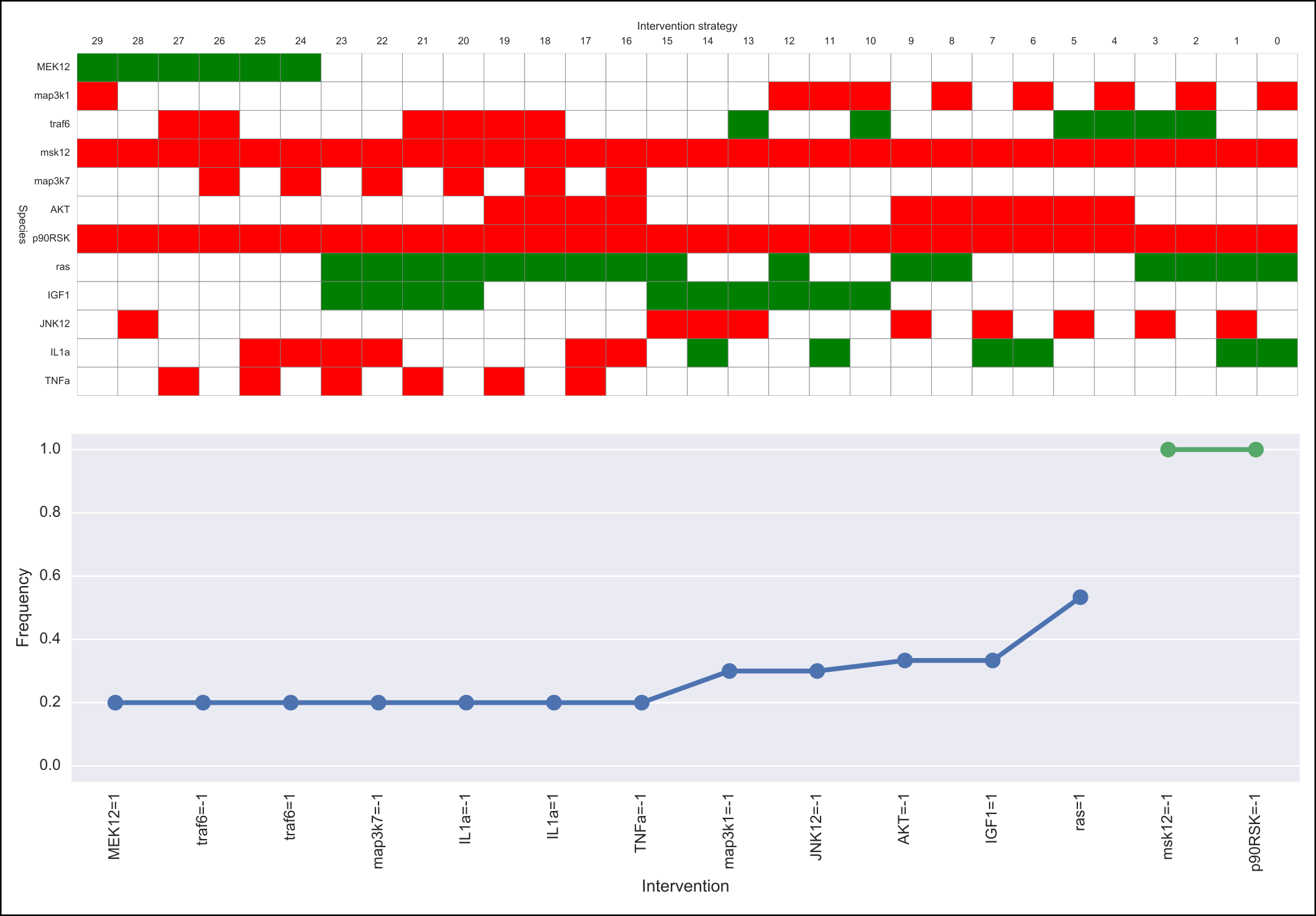
The output of caspo control will be two csv files, namely, strategies.csv and stats-strategies.csv. The file strategies.csv describes all intervention strategies found. The file stats-strategies.csv describes the frequency of each intervention over all strategies together with pairs of mutually inclusive/exclusive interventions. In addition, the following default visualizations are provided describing all intervention strategies:

Visualize

This subcommand implements all visualizations generated in other subcommands but to be run independently from the subcommand generating the data. This could be useful to visualize logical networks, experimental designs or intervention strategies not necessarily generated by caspo.

Help on caspo visualize:

$ caspo visualize --help
usage: caspo visualize [-h] [--pkn P] [--setup S] [--networks N] [--midas M T]
                       [--sample R] [--stats-networks F] [--behaviors B]
                       [--designs D] [--predictions P] [--strategies S]
                       [--stats-strategies F]

optional arguments:
  -h, --help            show this help message and exit
  --pkn P               prior knowledge network in SIF format
  --setup S             experimental setup in JSON format
  --networks N          logical networks in CSV format
  --midas M T           experimental dataset in MIDAS file and time-point
  --sample R            visualize a sample of R logical networks or 0 for all
                        (Default to -1 (none))
  --stats-networks F    logical mappings frequencies in CSV format
  --behaviors B         logical networks in CSV format
  --designs D           experimental designs in CSV format
  --predictions P       logical predictions in CSV format
  --strategies S        intervention strategies in CSV format
  --stats-strategies F  intervention frequencies in CSV format

Run caspo visualize:

$ caspo visualize --pkn pkn.sif --networks networks.csv --setup setup.json

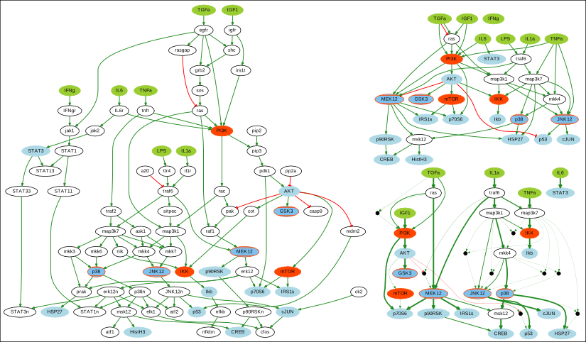
The output of caspo visualize will depend on the given arguments. Apart from the visualizations already shown when we described previous subcommands, it also provides visualization for a given PKN or a list of logical networks. Below we show an original PKN in the left, a compressed PKN in the top right, and the union of logical networks in the bottom right. Either all or a sample of logical networks can also be visualized individually using the --sample argument.

Note that PKNs and logical networks visualizations are generated as DOT files which can be either opened using a dot viewer or converted to different formats (pdf, ps, png, among others) using Graphviz. For example, you can convert from dot to pdf by running:

$ dot pkn.dot -Tpdf -o pkn.pdf

Test

Help on caspo test:

$ caspo test --help
usage: caspo test [-h] [--threads T] [--conf C]
                  [--testcase {Toy,LiverToy,LiverDREAM,ExtLiver}]

optional arguments:
  -h, --help            show this help message and exit
  --threads T           run clingo with given number of threads
  --conf C              threads configurations (Default to many)
  --testcase {Toy,LiverToy,LiverDREAM,ExtLiver}
                        testcase name

Run caspo test:

$ caspo test

Testing caspo subcommands using test case Toy.

Copying files for running tests:
    Prior knowledge network: pkn.sif
    Phospho-proteomics dataset: dataset.csv
    Experimental setup: setup.json
    Intervention scenarios: scenarios.csv

$ caspo --out out learn out/pkn.sif out/dataset.csv 10 --fit 0.1 --size 5

Optimum logical network learned in 0.0066s
Optimum logical networks has MSE 0.1100 and size 7
5 (nearly) optimal logical networks learned in 0.0075s
Weighted MSE: 0.1100

$ caspo --out out classify out/networks.csv out/setup.json out/dataset.csv 10

Classifying 5 logical networks...
3 input-output logical behaviors found in 0.2029s
Weighted MSE: 0.1100

$ caspo --out out design out/behaviors.csv out/setup.json

1 optimal experimental designs found in 0.0047s

$ caspo --out out predict out/behaviors.csv out/setup.json

Computing all predictions and their variance for 3 logical networks...

$ caspo --out out control out/networks.csv out/scenarios.csv

3 optimal intervention strategies found in 0.0043s

$ caspo --out out visualize --pkn out/pkn.sif --setup out/setup.json \
        --networks out/networks.csv --midas out/dataset.csv 10 \
        --stats-networks=out/stats-networks.csv --behaviors out/behaviors.csv \
        --designs=out/designs.csv --predictions=out/predictions.csv \
        --strategies=out/strategies.csv --stats-strategies=out/stats-strategies.csv

References

• [1] Exhaustively characterizing feasible logic models of a signaling network using Answer Set Programming. (2013). Bioinformatics.
• [2] Learning Boolean logic models of signaling networks with ASP. (2015). Theoretical Computer Science.
• [3] Designing experiments to discriminate families of logic models. (2015). Frontiers in Bioengineering and Biotechnology 3:131.
• [4] Minimal intervention strategies in logical signaling networks with ASP. (2013). Theory and Practice of Logic Programming.